lecture 5: Polynomial functions, their graphs, their domain and range, and their infinity behavior

What Are Polynomial Functions?

1. Real-World Motivation

Polynomials help model real-life situations with more complexity than just straight lines or parabolas.

Examples include:

• Profit modeling: $P(t) = -2t^3 + 9t^2 - 11t + 5$
• Population changes with limits or crashes
• Motion under forces (e.g., with acceleration, friction)

A polynomial is a function made by adding powers of $x$ with constant coefficients:

$$p(x) = a_n x^n + a_{n-1} x^{n-1} + \cdots + a_1 x + a_0$$

Where:

• $n$ is a non-negative integer (the degree)
• The $a_i$ values are real numbers

Why Study Polynomials?

• They are defined everywhere (no gaps or breaks)
• Easy to compute and graph
• Used as approximations in calculus (Taylor polynomials)
• Their graphs are smooth and continuous
• Appear in physics, engineering, economics, and more

Domain and Range

1. Domain

All polynomials are defined for all real numbers.

$$\text{Domain of any polynomial: } \mathbb{R}$$

2. Range

The range depends on:

• The degree (odd or even)
• The leading coefficient

We usually estimate range using the graph or calculus (later in the course).

Roots of Polynomials

1. What are Roots?

A root of a polynomial is a value of $x$ that makes the polynomial equal to zero.

2. How to find roots?

• Factoring: If $p(x) = (x-r_1)(x-r_2)\cdots(x-r_n)$, then $r_1, r_2, \ldots, r_n$ are the roots.
• Quadratic formula: For $ax^2 + bx + c = 0$, the roots are $x = \frac{-b \pm \sqrt{b^2 - 4ac}}{2a}$.
• Synthetic division: If $p(r) = 0$, then $r$ is a root. Then, $p(x) = (x-r)q(x)$ for some polynomial $q(x)$.

3. Example

Let:

$$f(x) = x^3 - 6x^2 + 11x - 6$$

• Roots: $x = 1, 2, 3$
• Factored form: $f(x) = (x-1)(x-2)(x-3)$

Graphing Polynomial Functions

1. Shape and Degree

The degree of a polynomial controls how many “turns” the graph can have.

Example of polynomials of different degrees:

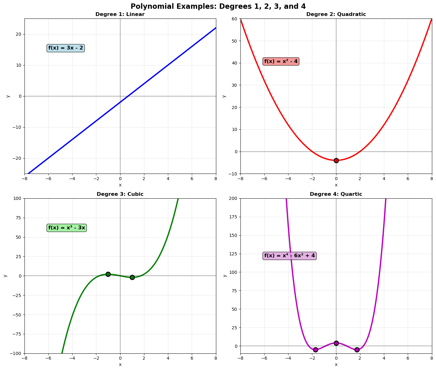
A degree-$n$ polynomial has at most $n-1$ turning points.

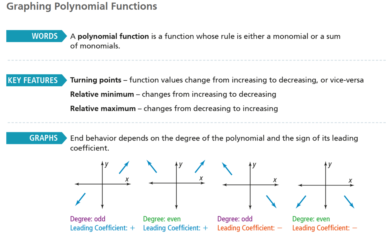
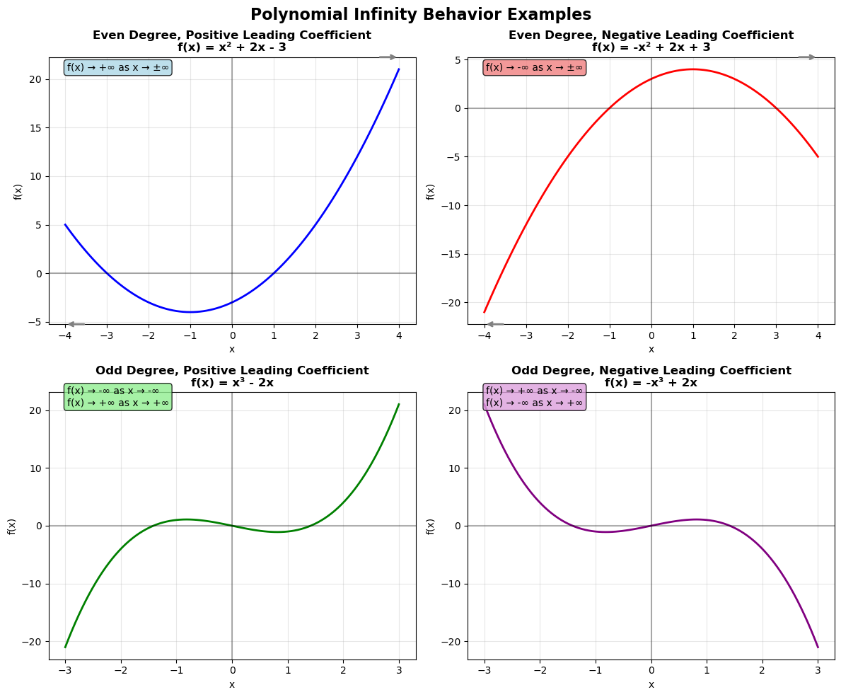
2. Infinity Behavior (a.k.a. End Behavior)

As $x \to \pm \infty$, the graph of the polynomial behaves like its leading term.

An infographic picture of polynomials behaviour at infinities:

Example with functions:

1. $f(x) = x^2 + 2x - 3$
2. $f(x) = -x^2 + 2x + 3$
3. $f(x) = x^3 - 2x$
4. $f(x) = -x^3 + 2x$

3. Example

Let:

$$f(x) = x^3 - 6x^2 + 11x - 6$$

• Degree: 3 (cubic)
• Leading coefficient: 1 (positive)
• Domain: $\mathbb{R}$
• Range: $\mathbb{R}$ (since degree is odd)

Turning Points: Up to 2
End Behavior:
$f(x) \to -\infty$ as $x \to -\infty$
$f(x) \to +\infty$ as $x \to +\infty$

Regular Exercises

1. Classify Polynomials

For each function, write the degree, leading coefficient, and whether it has an absolute maximum or minimum:

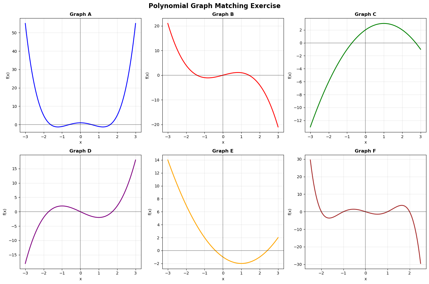
2. Match the Graph to the Function

Each of the following is a sketch of a polynomial. Without using a calculator:

• Decide if the degree is odd or even
• Determine if the leading coefficient is positive or negative
• Predict how many turning points it might have

3. Real-World Modeling

A company's profit over time is modeled by:

$$P(t) = -2t^3 + 9t^2 - 11t + 5$$

• a) What is the degree of this polynomial?
• b) What does the negative leading coefficient tell you about its long-term behavior?
• c) When might the company be losing money? (Estimate from the graph or table of values)

Solution
a) The function is:

$$P(t) = -2t^3 + 9t^2 - 11t + 5$$

The degree of a polynomial is the highest power of the variable. Here, the highest power is $t^3$, so the degree is:
Degree = 3

b) The leading coefficient is the coefficient of the highest degree term, which is −2.
Since it is negative and the degree is odd, the graph will rise to the left and fall to the right.
In other words, as $t \to -\infty$, $P(t) \to \infty$
and as $t \to \infty$, $P(t) \to -\infty$

This means that in the long run, the company's profits will decrease (possibly losses grow).

c) The company is losing money when $P(t) < 0$.
Without graphing exactly, we can estimate by plugging in a few values:

$$\begin{aligned} P(0) &= 5 \quad (\text{positive}) \\ P(1) &= -2(1)^3 + 9(1)^2 - 11(1) + 5 = -2 + 9 - 11 + 5 = 1 \quad (\text{positive}) \\ P(2) &= -16 + 36 - 22 + 5 = 3 \quad (\text{positive}) \\ P(3) &= -54 + 81 - 33 + 5 = -1 \quad (\text{negative}) \\ P(4) &= -128 + 144 - 44 + 5 = -23 \quad (\text{negative}) \end{aligned}$$

So the company begins losing money around $t = 3$ and continues downward afterward.

4. Design a Polynomial

Create a polynomial function that meets all of the following conditions:

• Degree = 3

• Positive leading coefficient

• Passes through the origin: $f(0)=0$

• Has a turning point somewhere between $x=1$ and $x=3$

  • a) Write a possible formula.
  • b) Sketch a rough graph.
  • c) What is the domain and range?

Solution
a) We want a degree 3 polynomial, with positive leading coefficient, that passes through the origin ($f(0) = 0$), and has a turning point between $x = 1$ and $x = 3$.

One possible function is:

$$f(x) = x(x - 1)(x - 3)$$

• Degree = 3 ✔️
• Leading coefficient = 1 (positive) ✔️
• $f(0) = 0$ ✔️
• Turning points occur near $x = 1.5$ ✔️

c)

• Domain: All real numbers, $\mathbb{R}$
• Range: All real numbers, $\mathbb{R}$ (since cubic polynomials have no upper/lower bounds)

5. Polynomial Passing Through Points

You are told a cubic polynomial passes through the following points:

• $f(0)=12$

• $f(1)=0$

• $f(2)=0$

• $f(3)=0$

• a) Write a possible formula for $f(x)$ in factored form.

• b) Expand the expression into standard form.

• c) What is the leading coefficient and what does it tell you about end behavior?

• d) What is the domain and range of your function?

Solution
a) We're told the function is cubic and passes through three x-intercepts (three roots):
$f(1) = 0$, $f(2) = 0$, $f(3) = 0$, and $f(0) = 12$

This suggests we can write the function in factored form:

$$f(x) = a(x - 1)(x - 2)(x - 3)$$

Use $f(0) = 12$ to solve for $a$:

$$f(0) = a(-1)(-2)(-3) = -6a = 12 \Rightarrow a = -2$$

So, the function is:

$$f(x) = -2(x - 1)(x - 2)(x - 3)$$

b) Expand the expression:
First expand two of the factors:

$$(x - 1)(x - 2) = x^2 - 3x + 2$$

Multiply with the third:

$$(x^2 - 3x + 2)(x - 3) = x^3 - 3x^2 + 2x - 3x^2 + 9x - 6 = x^3 - 6x^2 + 11x - 6$$

Multiply by $-2$:

$$f(x) = -2x^3 + 12x^2 - 22x + 12$$

c) The leading coefficient is −2

• Since the degree is 3 (odd) and the leading coefficient is negative, the end behavior is:
  • $x \to -\infty$, $f(x) \to \infty$
  • $x \to \infty$, $f(x) \to -\infty$

This tells us the function falls to the right and rises to the left.

d)

• Domain: All real numbers, $\mathbb{R}$
• Range: All real numbers, $\mathbb{R}$ (cubic polynomials are unbounded vertically)

Extra Advanced Exercises

1. Multiplicity Investigation

Consider the polynomial $f(x) = (x+2)^2(x-1)(x-4)^3$.

• a) How many real roots does this polynomial have?
• b) At which $x$-values does the graph of $f(x)$ cross the $x$-axis?

2. Turning Points Estimation

Suppose $h(x) = -x^4 + 4x^2$

• a) Find the x-intercepts of the graph of $h(x)$.
• b) Use symmetry and reasoning to estimate the turning points of the graph.
• c) What is the maximum value of $h(x)$?

3. Difference of polynomials

Let $f(x) = a_2x^2 + a_1x + a_0$.

• a) Compute $f(x+1) - f(x)$.
• b) What is the degree of the polynomial in part (a)?

Consider the polynomial $g(x) = b_nx^n + b_{n-1}x^{n-1} + \cdots + b_1x + b_0$.

• c) What is the degree of the polynomial $g(x+1) - g(x)$?